AWS Partner Network (APN) Blog
Transforming Geospatial Data to Cloud-Native Frameworks with Element 84 on AWS
By Matt Hanson, Sr. Software Engineer – Element 84
By Imtranur Rahman, Partner Solutions Architect – AWS
By Mary-Elizabeth Morin, Partner Development Manager – AWS
By Ariel Walcutt, Solutions Engineering Coordinator – Element 84
 |
| Element 84 |
 |
Element 84, in collaboration with Amazon Web Services (AWS) and Geoscience Australia, has released the Sentinel-2 Cloud-Optimized GeoTIFF (COG) dataset on AWS Open Data.
This includes a collection of all 11.4 million scenes from the Sentinel-2 Public Dataset, except for the JPEG2000 (JP2K) files which have all been converted to COGs. These datasets are continuously updated to mirror the growth of the public Sentinel-2 data, and we have added SpatioTemporal Asset Catalog (STAC) metadata to the JSON file to make searching, discovering, and working with the data easier.
Sentinel-2 is an important platform for Earth observation, and its imagery contributes to ongoing research in climate change, land use, emergency management, and a host of other geophysical systems.
There are two Sentinel-2 satellites—Sentinel-2A and Sentinel-2B—both in sun-synchronous polar orbits, 180 degrees out of phase from one another. This allows the system to cover the entire planet with a revisit time (the time it takes for the satellite to get back over a previously-imaged area) of five days in mid-latitudes.
Sentinel-2 imagery is great for detecting changes on the Earth’s surface (think: last week there were trees here, this week they are gone) and is a key tool for evaluating geographic areas before and after natural disasters.
Element 84 is an AWS Advanced Consulting Partner and a founding member of the AWS Public Safety and Disaster Response Competency, working with business and government to create applications and data systems that help users solve problems or answer big questions. Element 84 designs, develops, and operates scalable software solutions that help customers understand our changing planet.
The 2020 North Complex Fire devastated California’s Berry Creek region. In this post, using STAC technologies and resources on the Registry of Open Data on AWS, we analyze and visualize ESA Sentinel-2 data to demonstrate the capability of these tools to accelerate time to insight. This can help disaster response organizations focus on saving lives, not wrangling data.
By making the Sentinel-2 archive more cloud-native via COGs and STAC, we are making the data more user-friendly and (hopefully) making the lives of emergency managers, climate scientists, and policy makers that much easier. This is a small step in our big goal of doing work that benefits the world while enabling us to scale up to hundreds and thousands of datasets in cloud.
Solution Architecture
The following diagram represents an overview of the solution. We will be using Amazon Elastic Kubernetes Service (Amazon EKS) to deploy a DASK cluster using Helm chart. Then, with the help of a JupyterHub notebook deployed as part of the DASK cluster installation, we’ll pull the Sentinel image data stored in an Amazon Simple Storage Service (Amazon S3) bucket, process it, and use it in our solution.

Figure 1 – Solution architecture.
Prerequisites
- AWS account with admin privileges.
- Command line tools. Mac/Linux users need to install the latest version of AWS Command Line Interface (CLI), kubectl, Helm, and eksctl on their workstation. Windows users need to create an AWS Cloud9 environment and then install these CLIs inside their Cloud9 environment.
- DASK cluster in the same AWS Region as that of the data (us-west-1).
- Amazon SageMaker and Jupyter with Python 3 kernel and the following packages installed:
- geopandas, scikit-learn, statsmodels, seaborn, cartopy, pystac-client, stacterm, hvplot, rasterio, geoviews, rioxarray, fsspec, s3fs, requests, aiohttp, odc-algo.
Step 1: Create Amazon EKS Cluster
For the purpose of this post, we’ll create an Amazon EKS cluster using eksctl. To begin, create a yaml file in your home directory, copy and paste the following text, and then save the file.
Note: You can skip this step if you already have an EKS cluster running.
To create a cluster, run the following command:
After your cluster is up:
- Update the local kubconfig using the following command:
- To test connectivity, run the following command:
You should see output similar to that of Figure 2. If you don’t see similar output, you haven’t updated the config properly.

Figure 2 – kubectl get node output.
Step 2: Add the DASK Helm Repo and Deploy the DASK Cluster on Amazon EKS
To add the Dask community Helm charts for the Kubernetes repo, and then deploy the chart on EKS, run the following commands:
After successful deployment of the Helm chart, you should see output similar to Figure 3:

Figure 3 – DASK cluster deployment output.
This chart will also deploy a Jupyter notebook for you on the cluster. However, you can use any other notebook Integrated Development Environment (IDE), such as Amazon SageMaker, for this.
To access the Jupyter notebook (deployed with Helm) from your local machine, run the following commands:
Next, open a web browser and access the URL: http://localhost:8082. Locate the password from the Helm output and use it to log in to the Jupyter notebook.
After successful login, you should see the Jupyter notebook.
Step 3: Start the Data Transformation Using pystac-client
In this step, we’ll use the pystac-client library to query Earth-Search for Sentinel-2 satellite data, exploring the metadata returned, and then later access the image data.
Using Pandas, GeoPandas, and hvPlot, we’ll show how to visualize geospatial data, make simple plots of the metadata, and render the imagery as an interactive time series. Earth-Search is powered by Element84 stac-server, a STAC-compliant API deployed as an AWS serverless app backed by Elasticsearch.
Start with a spatial area of interest (AOI), defined as a single GeoJSON having a geometry type of Point, LineString, Polygon, MultiPoint, MultiLineString, or MultiPolygon.
Note: GeometryCollection is not supported.
To create an AOI of your own, use http://geojson.io/ and create a single GeoJSON Feature:
- Copy the GeoJSON data from the above URL and save the single Feature (not the whole FeatureCollection) in a file accessible by your code inside the Jupyter notebook. For this post, we have selected Berry Creek California GeoJSON.
.

Figure 4 – GeoJSON of area of interest.
- Inside your Jupyter console, select Text File, paste the copied GeoJSON, select File > Save as, and enter a name for the file.
- To use this file, we need to know its path. To get the path, right-click the file and select Copy Path.
.
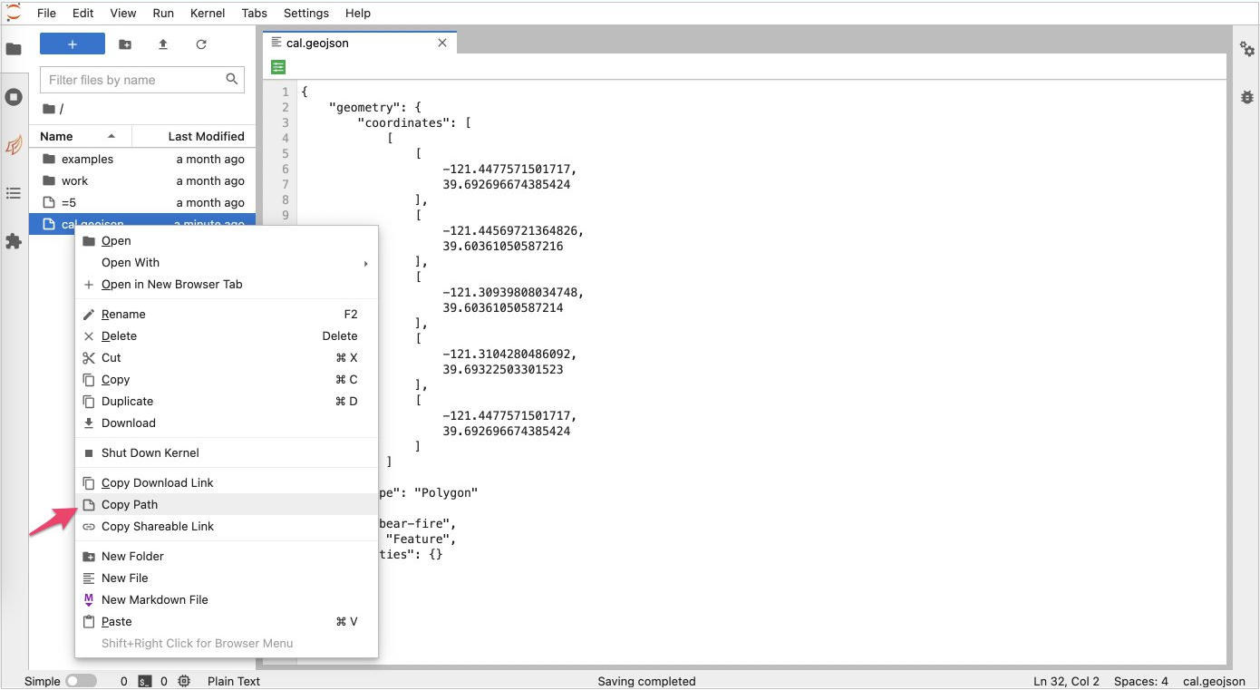
Figure 5 – Copy GeoJSON file path.
- Paste the path value in “filename = <>” in the following code snippet.
- Copy the code from the following snippet, paste it in the Jupyter notebook cell, and then run the commands by choosing Shift + Enter.
After running these commands, you’ll see an image in the Jupyter notebook that shows the footprint of our area of interest on top of an open street map on the base layer.

Figure 6 – Footprint of AOI on map.
Querying Earth-Search: The preceding AOI geometry can be used with an intersects argument to locate data whose footprint intersects with it. In the following code, the geometry is loaded.
Using the STAC API query extension, we’ll query the STAC Item property. We are then going to limit the query to images with data covering most of the tile, rather than working with scenes containing a large portion of “no data” values.
Here, we are looking for scenes that have a calculated cloud cover (sentinel:valid_cloud_cover=true) that is less than 10% covered by clouds (eo:cloud_cover<=5).
- To run this query, copy the following code snippet, paste it in the Jupyter notebook cell, and then choose Shift + Enter.
- Now, with the pystac_client module’s Client class, we’ll open STAC API. Then, using the search function with our parameters, we’ll fetch all of the items. To run this search, copy the following code snippet, paste it in the Jupyter notebook cell, and then choose Shift + Enter.
You should see output similar to that of Figure 7:
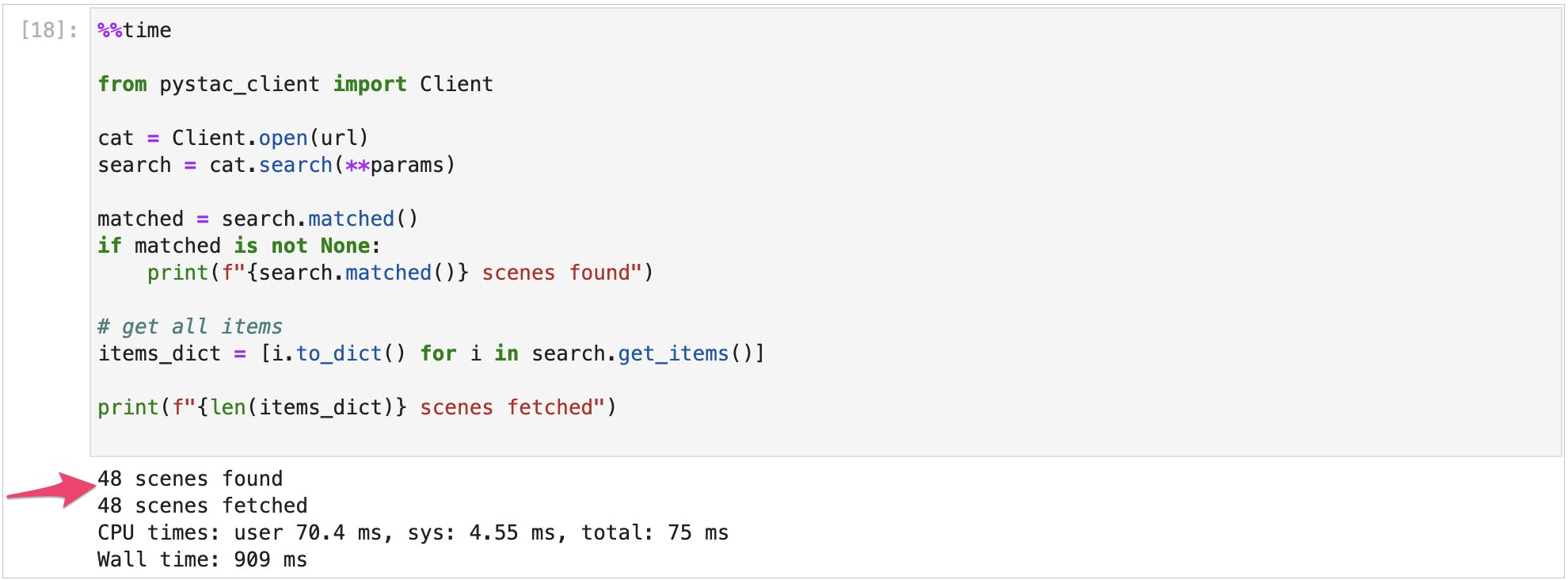
Figure 7 – Number of scenes.
Metadata visualizations: To explore and visualize the items, let’s load them into a GeoDataFrame with the items_to_geodataframe function. This will properly load the geometries to the Geometry type, convert datetime to datetime objects, and set the index of the GeoDataFrame to datetime (the image acquisition datetime).
Similar to the preceding AOI visualization, we can view the geometry footprints of the found STAC items along with our AOI by plotting the items and using the HoloViews overlay (*) operator to show the AOI with it in a different color.
The map shows the footprint of all the STAC items in blue, which because they all cover the same area at different points in time appears as a single shape. The red rectangle is the AOI, which is far smaller than the data tiles. It would be a shame if we had to download an entire tile of data for every spectral band we wanted, since it’s a lot of extra data we won’t use.

Figure 8 – Footprint of all the STAC items.
Exploring the data with Pandas: With the STAC items in a GeoDataFrame, we can view the geometries on a map as above, but there is more that can be done to visualize and explore the data.
Look at the first few rows of the GeoDataFrame (each row is a STAC item), and you’ll see the JSON has been normalized so each field in a nested dictionary (such as assets) is its own column. There are many columns, so we’ll print all of the column names except for the assets (the datafiles themselves), which we’ll look at later.

Figure 9 – STAC items.
As with viewing the geometry, hvPlot can also be used to plot numeric fields. The Sentinel-2 data does not have many useful numeric properties except for eo:cloud_cover and sentinel:data_coverage.
Because low data coverage was filtered out in the above search, we expect to see high data coverage over all scenes, which we do—they all have 100% coverage.
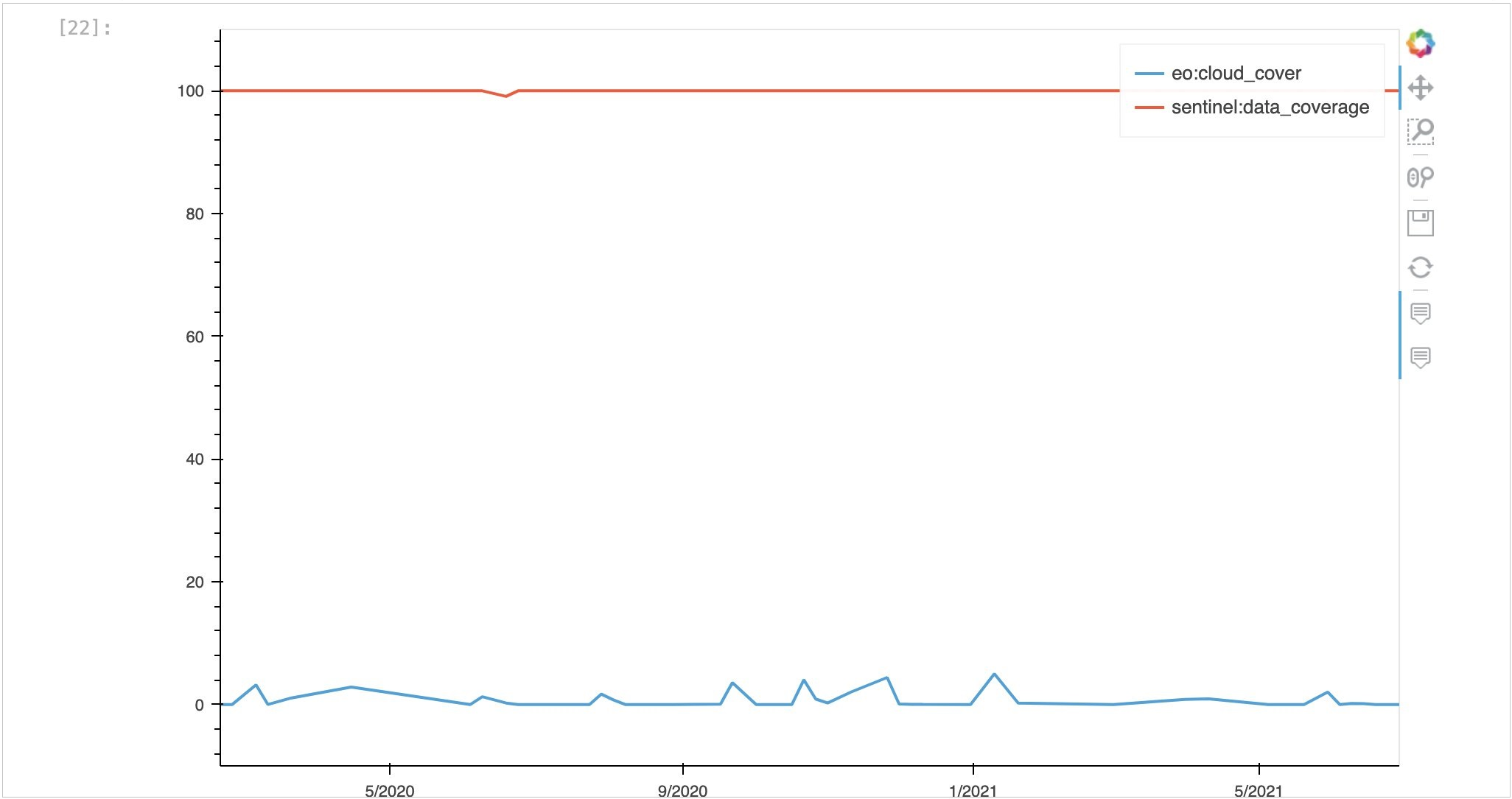
Figure 10 – Data coverage plot.
Step 4: Data Access
So far, we have only looked at metadata. We haven’t looked at any data. Before data access, you need to understand the assets available using Pandas.
xarray
The stackstac library helps create xarrays (labeled numeric arrays) from STAC item assets. Open all of the items as an xarray, specifying the red, green, and blue bands only.
Figure 11 shows the constructed XArray from the stack of STAC items. There are 48 time slices, each composed of a 3-band image that’s just under 11K x 11K pixels in size.

Figure 11 – xarrays from STAC item assets.
We are only interested in the above AOI, so we’ll use rioxarray to clip the full xarray down to our polygon. To do so, run the following commands:
Running these commands is a necessary precursor before the user can visualize the data in the next step, thus reducing the total data load.

Figure 12 – Clipped full xarray down to AOI polygon.
Now, it’s time to fetch all of the data and apply any processing by calling the compute function that turns the virtual Dask arrays into real arrays.
Although the Dask cluster can be used on any machine, it’s more efficient to use a Dask cluster deployed on Amazon EKS and located next to the data. Connect to the Dask cluster deployed in us-west-2 for fast access to the Sentinel-2 data. The cluster will read and process the data, delivering the final arrays to your code.

Figure 13 – Final array.
To visualize the data, run the following commands to scale the data and create an RGB image:
Next, we’ll use the cluster to fetch the data and apply all the processing to it:
Using the DASK cluster running on EKS, we’ll generate byte-scaled data that can be displayed as a true color image (using the red, green, blue bands), as shown in Figure 14.

Figure 14 – True color image of Byte scaled data.
Finally, we’ll visualize the data as RGB images with a time slider for moving through the time series.
The resulting true color image highlights drastic impacts on the Berry Creek region caused by the Bear Fire, including significant burnt vegetation.
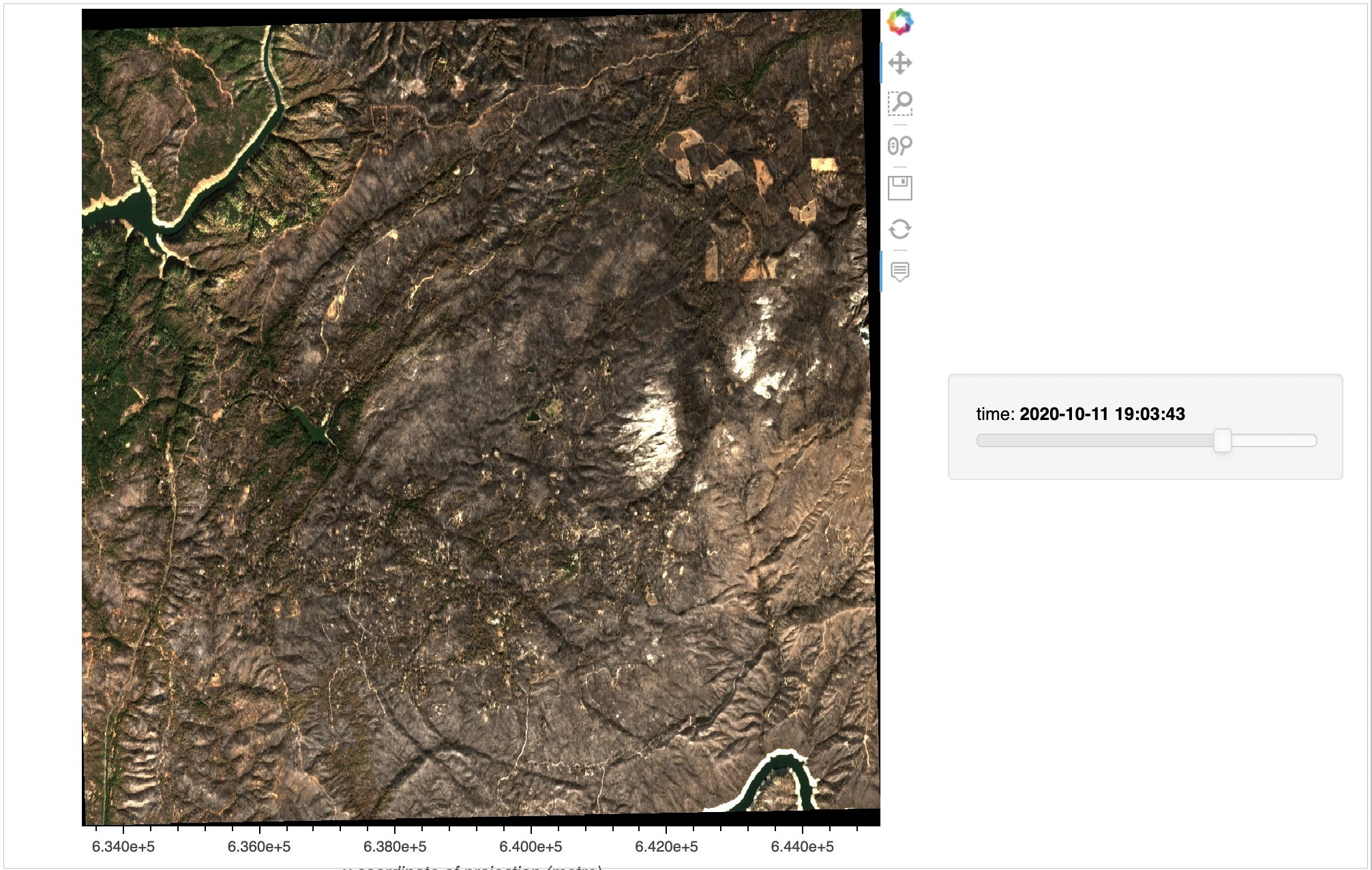
Figure 15 – True color RGB image with Time Slider.
Optionally, we can create an animated gif of the sequence:
The generated gif shows that lush vegetation is decimated by the wildfire, resulting in a burnt landscape.

Figure 16 – True color RGB image in GIF.
Step 5: Cleanup
To clean everything up, run the following command to find the helm release installed:
To remove that release, run helm uninstall:
Conclusion
In this post, we have identified an area of interest (AOI) encompassing Berry Creek, California, and using its geometries we queried, fetched, and analyzed data using a Dask cluster deployed on Amazon EKS and Jupyter notebook.
We visualized data from the Sentinel-2 Cloud-Optimized GeoTIFF dataset using STAC tooling, and created an animated gif which shows the destruction of the North Complex Fire engulfing Berry Creek.
This entire workflow can be performed in the cloud without the need to download or process the Sentinel-2 data locally. Cloud-optimized data and workflows greatly reduce the “time to science” and let researchers spend more time analyzing and less time wrangling their data.
.

.
Element 84 – AWS Partner Spotlight
Element 84 is an AWS Competency Partner that works with business and government to create applications and data systems that help users solve problems or answer big questions.
Contact Element 84 | Partner Overview
*Already worked with Element 84? Rate the Partner
*To review an AWS Partner, you must be a customer that has worked with them directly on a project.