AWS HPC Blog
Getting the best OpenFOAM Performance on AWS
OpenFOAM is one the most widely used Computational Fluid Dynamics (CFD) packages and helps companies in a broad range of sectors (automotive, aerospace, energy, and life-sciences) to conduct research and design new products. Its open-source nature means it’s particularly suited to the cloud because end users can take advantage of the flexibility and scale of the compute resources on AWS without being constrained by license limits. For the same reason, OpenFOAM has increasingly become the code of choice to power software as a service (SaaS) solutions, where a custom web interface lets customers submit their job with little effort.
In this post, we’ll discuss six practical things you can do as an OpenFOAM user to run your simulations faster and more cost effectively.
This post focuses on a relatively simple OpenFOAM case (a 35M cell motorbike model). In future posts we’ll show a similar analysis for more complex models.
Our test environment
OpenFOAM comes with multiple tutorials that show you how to use its various solvers and to setup your workflows. Unfortunately, most are too small to be used to understand HPC performance because they’re designed to run on your laptop or workstation. This has led to users creating larger cases, with higher mesh counts to test performance on HPC clusters. But just matching the number of cells can give vastly different results if a different case setup is used.
The OpenFOAM HPC technical committee (of which AWS is a member) was created to standardize this and provide a consistent approach. The committee has created a series of test-cases (available on GitLab) that can be used by the community to test OpenFOAM’s HPC performance in a transparent way. In this post we’ll use the largest variant of the motorbike test-case using approximately 35M cells.
All our simulations used OpenFOAM v2012, but the majority of the proposals and discussion here should work equally well for other versions and branches of OpenFOAM.
We’ve used the HPC environment from the AWS CFD workshop series. At the time of our tests:
- AWS ParallelCluster HPC deployment tool (version 3.0.3)
- Amazon Linux 2 operating system
- Intel MPI 2019.8 for x86 and Open MPI 4.1 for Graviton2 instances
- Amazon FSx for Lustre parallel file-system (4.8TB SSD-based)
- A range of Amazon EC2 instances
- Elastic Fabric Adapter (EFA) network adapter (as well as TCP for our non-EFA enabled instances)
The base case: a typical OpenFOAM workflow
Many OpenFOAM users base their CFD workflow on the tutorials that come with OpenFOAM. The process depends on whether they’re using the in-built mesher snappyHexMesh or an external tool such as ANSA or Pointwise. For this post, we’ll focus on the snappyHexMesh-based workflow.
The meshing and solving is typically done on the same number of cores. We want to explore how the performance of this looks for a 35M cell motorbike case. We’ll use the unmodified case from GitLabexcept for the order of the commands (it’s assumed in the GitLab version that the case is meshed and then redistributed to serial and then decomposed back to the number of cores we want to run on).
To provide a scalable way to increase the case size, the difference between the S, M and L versions of this case are that the motorbike itself (8M cells) is mirrored to create larger meshes. This is done once for the medium case (~18M cells) and twice for the L (~35M cells) so there are actually four motorbikes in the L case. Since the mirroring time is minimal, we excluded it for this analysis, which means the meshing time reported is just the snappyHexMesh time for the 8M cell model.
Importantly, for this test case the linear solver is the DICPCG solver i.e., Preconditioned Conjugate gradient-type approach. This differs from the multi-grid method that is typically used for external aerodynamics cases in OpenFOAM. Future posts will look at comparing the two linear solvers for a more complex case.
Discussion
1. Core Counts
Figure 1 shows that the total simulation time (blockMesh, decomposePar, snappyHexMesh, potentialFoam and simpleFoam processes combined) using the Amazon EC2 c5n.18xlarge instance (more details in Table 1) doesn’t speed up any further after 288 cores (8 nodes), which is approximately 120,000 cells per core. Cells per core is a useful metric because it allows us to extrapolate to other cases (i.e., divide the size of the mesh by cells-per-core to reach optimum number of cores to run on) and incorporates the idea of there being a cross-over between when a certain number of cells on a processor goes from being mainly memory-bandwidth limited to also being limited by network communication across the cores and nodes. If we dig deeper, we can split out the time for the two most significant parts of the process (e.g. snappyHexMesh and simpleFoam) shown in Figure 2 and 3. To see the variation away from linear scaling a ‘scale-up’ parameter is used:

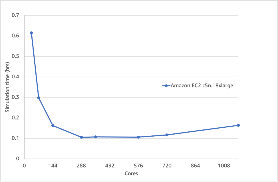
Figure 1 – Overall simulation time (solve + mesh) of the 35M cell motorbike case which doesn’t speed up after 288 cores
The simpleFoam ‘solver’ part is linear up to ~900 cores (~40,000 cells per core) whereas the snappyHexMesh meshing phase does not even scale linearly to two nodes (~200,000 cells per core – based upon 8M cell snappyHexMesh model). Running on the same number of cores for the meshing, solve and post-processing phase is not a good idea, because snappyHexMesh can’t scale as well. This influences the overall scaling and means that practically you can’t run more than 288 cores.
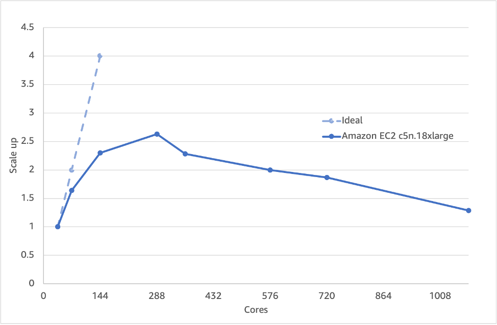
Figure 2 – Scaling of the snappyHexMesh portion of the 35M cell motorbike case which doesn’t scale past 72 cores
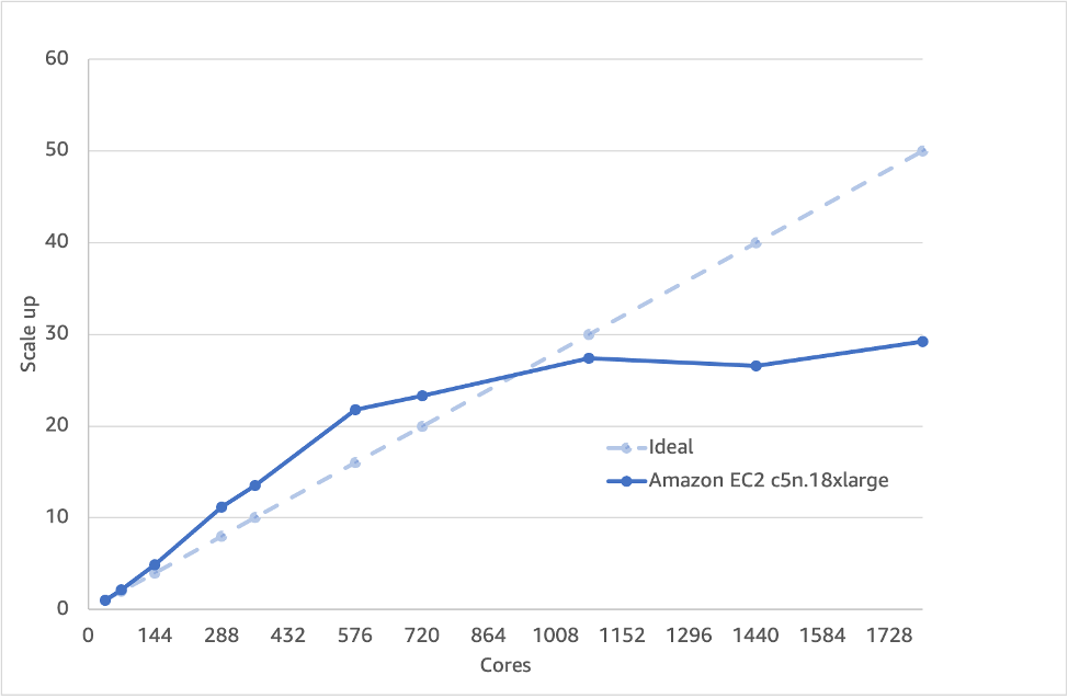
Figure 3 – Scaling of the simpleFoam solver portion of the 35M cell case
One option is to run the meshing and solve phase on a different number of cores. Let’s explore that new workflow idea and use the opportunity to look at the influence of different Amazon EC2 instance types, as well.
Recommendation 1: Don’t run the same number of cores for your snappyHexMesh and solve (e.g simpleFoam)
2. Meshing optimization
AWS currently has more than 475 instance types which are designed for a diverse range of workloads. For CFD there are six instance types that customers tell us they use the most. These are shown in Table 1. While we explore the performance of the meshing phase (Figure 4) we can start to bring in the impact of cost using the AWS On-Demand Instances pricing model (Figure 5).
Table 1 – Amazon EC2 instances used in this blog
| Instance | Details |
| C5n.18xlarge | Intel Xeon Skylake 36 cores @ 3.5GHz, Memory: 192GB – 100Gbit/s EFA |
| C6g.16xlarge | Arm-based Graviton2 64 cores @ 2.4GHz, Memory 128GB – 25Gbit/s TCP |
| C6gn.16xlarge | Arm-based Graviton2 64 cores @ 2.4GHz, Memory 128GB – 100 Gbit/s EFA |
| C5.18xlarge | Intel Xeon Skylake 36 cores @ 3.2GHz, Memory: 192GB, 25Gbit/s TCP |
| C6i.32xlarge | Intel Xeon Icelake 64 cores @ 3.5GHz , Memory 256GB, 50Gbit/s EFA |
| Hpc6a.48xlarge | AMD EPYC Milan 96 cores @ 3.6GHz, Memory 384GB, 100 Gbit/s EFA |
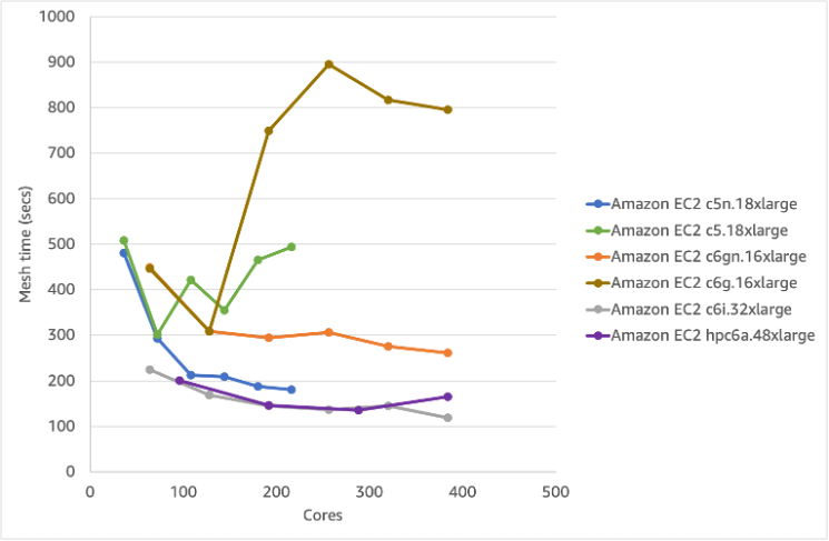
Figure 4 – Performance and scaling of various EC2 instances for the snappyHexMesh phase (lower is better)
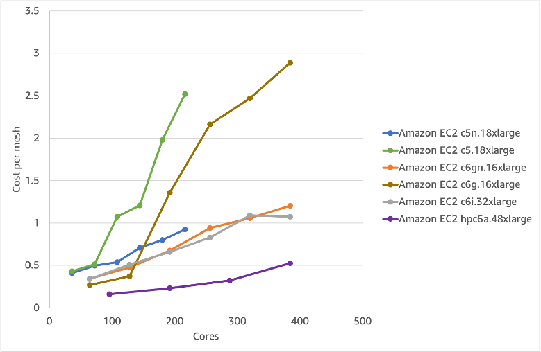
Figure 5 – Cost per mesh using various EC2 instances (on-demand pricing)
The latest generation AMD Milan Hpc6a.48xlarge and Intel Icelake c6i.32xlarge gives the best performance. The lowest cost option is however the Hpc6a.48xlarge which is our first HPC-optimized Amazon EC2 instance. Interestingly, the graph shows just how sensitive snappyHexMesh is to the network adapter: both non-EFA options (c6g.16xlarge and c5.18xlarge) perform worse and cost more per mesh, than the EFA-enabled versions.
Recommendation 2: Use EFA enabled instances for the snappyHexMesh phase and aim for > 100,000-200,000 cells per core
3. Domain Decomposition
Diving even deeper let’s look at one of the most impactful software changes: the method of domain decomposition. We essentially have two approaches: (1) hierarchical, where we manually specify the split in the x, y and z directions; or (2) scotch, where we allow the method itself to decide how best to split up the domain. Figure 6 shows the effect domain decomposition choice has on the speed and scaling of the snappyHexMesh process. First, the scotch method is approximately 2x slower than hierarchical when we go past 64 cores, and it scales poorly compared to the hierarchical approach. This is independent of the AWS instance choice. Approximately 100 cores is the sweet spot of price/performance for meshing using the hierarchical domain decomposition approach for this case.
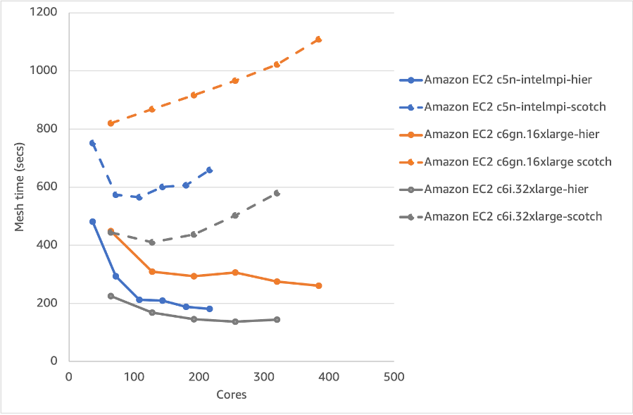
Figure 6 – Meshing time for various EC2 instances for scotch and hierarchical domain decomposition
Recommendation 3: Use the hierarchical method for the meshing domain decomposition
4. Solver performance
Let’s repeat the performance/price optimization that we did for meshing. However, let’s first look at the difference between hierarchical and scotch domain decomposition for the simpleFoam portion of the job. Figure 7 shows that for this setup the performance is very similar during the linear (or indeed super-linear) part of the graph. But once network communication becomes the bottleneck (rather than memory bandwidth or cache effects) at around 576 cores, scotch becomes the better option. This is because the load balancing approach of assuming a certain spatial distribution of cells to each processor is unlikely to be as good as one which has been optimized based upon the grid itself. In future posts, we’ll show that this makes a big difference when we use the multi-grid option for a more complex case setup.
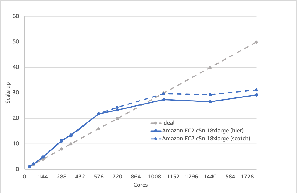
Figure 7 – Scaling of the simpleFoam part using different domain decomposition approaches
Recommendation 4: Use scotch for the solve (e.g simpleFoam) domain decomposition
5. Solver Instance Choice
We’ll use scotch as the domain decomposition method in the assessment of different EC2 instances. Figures 8 and 9 show that the performance per-core and per-node is very much dependent on the instance selection with the c6i.32xlarge offering the best performance per-core. There is also a clear benefit to using EFA, where non-EFA options (c6g.16xlarge and c5.18xlarge) show worse scaling performance than their EFA-enabled versions. However, the difference between Figure 8 and 9 is important. Traditionally many CFD users have focused on per-core performance. Since on AWS you ultimately pay for an instance, it’s useful to also compare on a per-node basis. In this way, we can see that options like hpc6a.48xlarge are more competitive to the other instances, despite looking slower in Figure 8 because of the higher number of cores per node. In reality this means you sometimes need to run more cores for a particular node type than another to get the same performance or under-populate and run fewer cores per node. This is something we’ll cover in a future post on hpc6a.48xlarge, which can show similar results to c6i.32xlarge when using 48 or 72 cores per node for certain workloads.
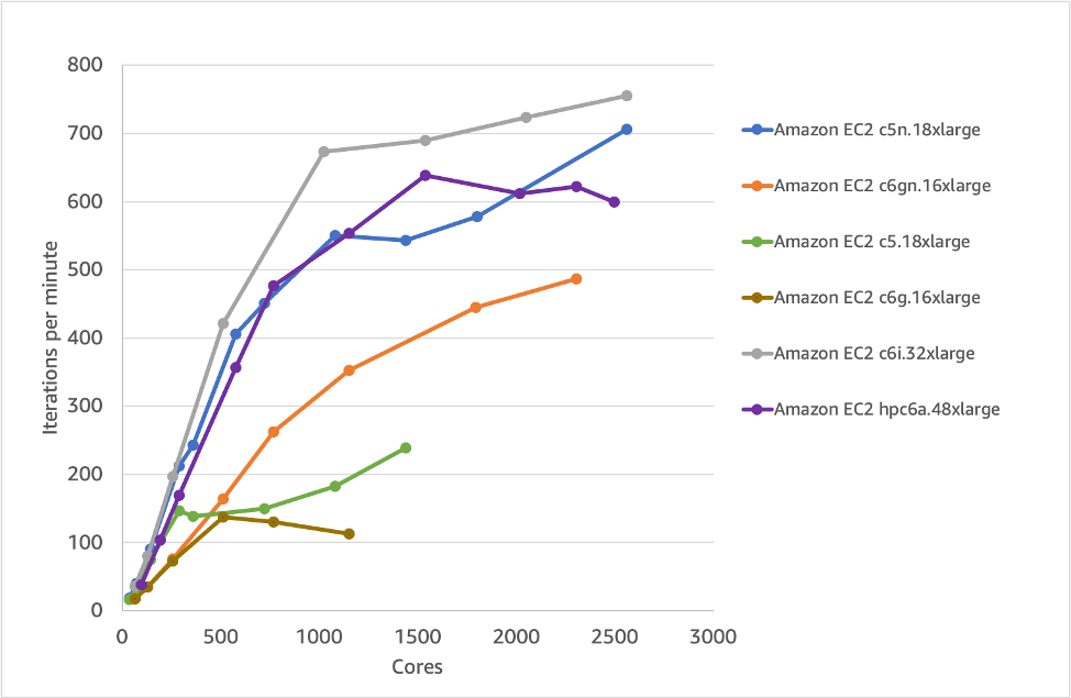
Figure 8 – Scaling of various EC2 instances for the simpleFoam portion of the simulation
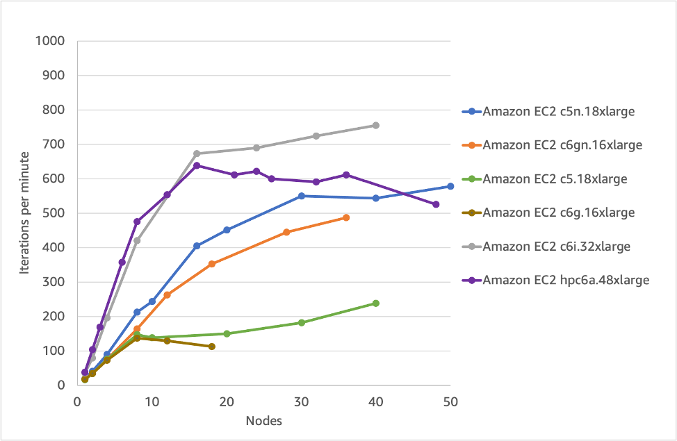
Figure 9 – Scaling of various EC2 instances for the simpleFoam part (per-node)
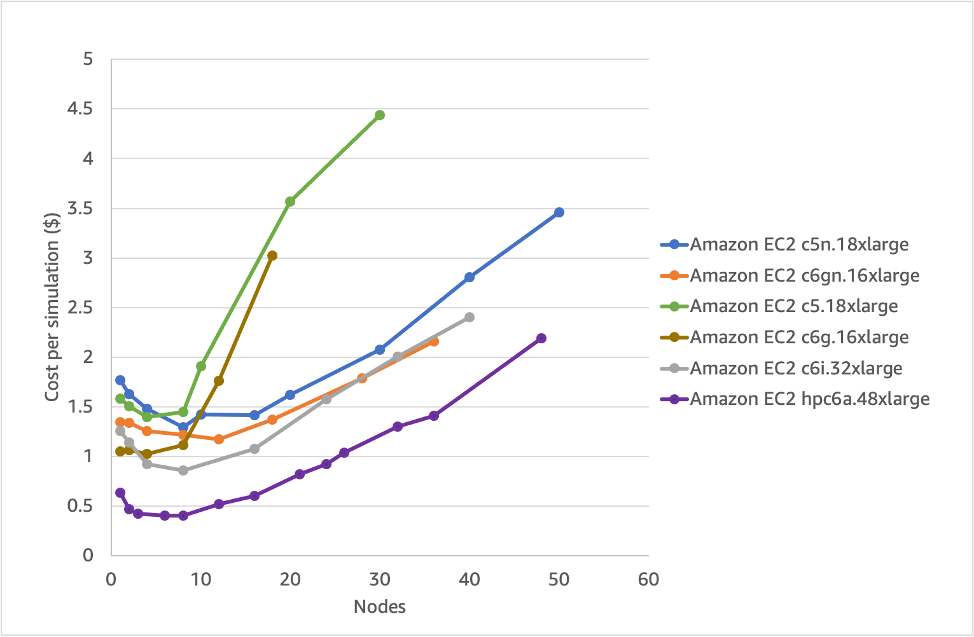
Figure 10 – cost per simulation (on-demand pricing) for various EC2 instances (lower is better)
As with the snappyHexMesh analysis, a key metric is the cost. Figure 10 shows this for the various EC2 instances types. The optimum instance that minimizes the cost is clearly hpc6a.48xlarge. Combining Figures 9 and 10 means we can pick the right instance type depending on whether we want to prioritize price, performance or a middle-ground. Although the optimum price/performance per-core option was ~100 cores for meshing, the simpleFoam part shows an optimum price around 650 cores (depending on the instance type).
Recommendation 5: Consider HPC-optimized instances for the best-price performance and aim for 50,000-100,000 cells per core
6. A new workflow
Key questions remain about how to move from the meshing phase to the solver phase (when using a snappyHexMesh based workflow), and how to move between hierarchical and scotch domain decomposition techniques. The approach in the original version of this case is to redistribute after meshing back to serial and then decompose back to the required number of instances. This is what many OpenFOAM users still do. It can work fine if you generate a grid once but if mesh generation is part of every run (like when designing a car or a plane) this approach isn’t great.
This is particularly true when we get to larger meshes of more than 100M cells, where reconstructing the mesh back to serial, and then re-partitioning, can take many hours and require more RAM than is available in a typical instance. In our example here, it took consistently 5 minutes (it’s a serial process), which is the same amount of time as for meshing. But while you might be able to mesh on larger cores to keep the time down, the process of redistributing back to serial stays constant at several hours for large cases.
A better option is to use the redistributePar option which can, in parallel, move from a set number of cores to a different number and at the same time change the decomposition method (if required).
We can also split up our submission script into two parts and, using dependencies, submit both jobs at once, linking them together. This means the solve part will only run once the meshing is complete. We then have the freedom to choose different cores, instance types and domain decomposition for each part. Since a single AWS ParallelCluster can have multiple queues, each with different instance types and sizes, we can easily optimize each part of the workflow.
Recommendation 6: Using ‘dependencies’ to submit your jobs to run on different cores and instance types for meshing and solve using the parallel reconstructPar approach
Conclusion
In this post, we examined six key variables, covering both software and hardware, to find the optimum price, performance (or both) for running OpenFOAM simulations. We started with a base case: meshing and solving on the same number of cores, on the same processor type and with one domain decomposition method. Hopefully you’ll now agree that a better approach is to split the job into different processes and processors so we can apply different core-counts and different architectures to the various workflow steps. We can achieve the most efficient price/performance by using different queues with difference instance types, each optimized for separate parts of the problem.
We’re always working on new instance types and families, so we’ll update this advice often. You can stay up to date by following this blog channel. The AWS CFD page also has links to OpenFOAM-specific workshops that guide you step-by-step to from new account and all the way to running your OpenFOAM jobs.
Please also watch out for futures posts that will provide further things you can do to optimize price and performance for more complex cases.