AWS for Industries
Exploring the UniProt protein knowledgebase with AWS Open Data and Amazon Neptune
Example graph of protein data
The Universal Protein Resource (UniProt) is a widely used resource of protein data that is now available through the Registry of Open Data on AWS. Its centerpiece is the UniProt Knowledgebase (UniProtKB), a central hub for the collection of functional information on proteins, with accurate, consistent and rich annotation. UniProtKB data is highly structured with many relationships between protein sequences, annotations, ontologies and other related data sources. UniProt can be directly accessed via the UniProt website and is available for bulk downloads in several formats, including RDF which is particularly well suited to represent the complex and connected nature of the data as a graph. Creating a custom knowledgebase can enable more advanced use cases, such as joining with other data sources, augmenting data with custom annotations and relationships, or inferring new relationships with analytics or machine learning.
In this blog post, we demonstrate the step-by-step process to create and use your own protein knowledgebase using UniProt RDF data. We will show how to ingest a subset of UniProtKB data into your own Amazon Neptune database directly from the Registry of Open Data on AWS. We then show how to query the data with SPARQL, create new relationships in the data, and visualize the data as a graph.
Registry of Open Data on AWS
The Registry of Open Data on AWS makes it easy to find datasets made publicly available through AWS services. UniProt is made available through the Registry of Open Data via the Open Data Sponsorship Program, which covers the cost of storage for publicly available high-value cloud-optimized datasets. UniProt is available in the registry as RDF files, a standard model for data interchange on the Web that is capable of capturing complex relationships within the data of the UniProtKB. To look for other datasets or learn more on publishing datasets, visit the registry of open data on AWS.
Amazon Neptune
Amazon Neptune is a fast, reliable, fully managed graph database service that makes it easy to build and run applications that work with highly connected datasets. The core of Neptune is a purpose-built, high-performance graph database engine. This engine is optimized for storing billions of relationships and querying the graph with milliseconds latency. Neptune supports the popular graph query languages Apache TinkerPop Gremlin and W3C’s SPARQL, enabling you to build queries that efficiently navigate highly connected datasets.
Creating a custom UniProtKB
In this example, we select a list of UniProt RDF files that we are interested in exploring. Then we ingest the RDF files from the Open Data Registry on AWS into Amazon Neptune DB. Once the data is ingested, we demonstrate how to query relationships and attributes. By adapting this example to your own research needs, you should be able to build a subset of UniProtKB containing data for your specific use case. This example will also be the foundation of our follow-on example where we will use Neptune ML to predict relationships and attributes in the UniProtKB.
Brief overview of UniProt data
UniProt RDF files are located in a public S3 bucket s3://aws-open-data-uniprot-rdf. There are different paths for each data release. New data releases typically happen every two months, so be sure to use the latest release directory. We use the first release of 2021, which has a path of s3://aws-open-data-uniprot-rdf/2021-01. For more information on the data, see the UniProt help pages. Here is a brief description for some of the different datasets and files:
Taxonomy, Gene Ontology (GO) and other reference data
UniProt uses several supporting reference datasets that contain related information and metadata. Among these are the NCBI taxonomy, for the hierarchical classification of organisms, and the Gene Ontology (GO), used to describe the current scientific knowledge about the functions of proteins. The GO is represented with the Web Ontology Language (OWL), which is used to define ontologies that describe taxonomies and classification networks, essentially defining the structure of a knowledge graph. OWL is also built upon RDF.
| File | Description |
| citations.rdf.gz | Literature citations |
| diseases.rdf.gz | Human diseases |
| journals.rdf.gz | Journals which contain articles cited in UniProt |
| taxonomy.rdf.gz | Organisms |
| keywords.rdf.gz | Keywords |
| go.rdf.gz | Gene Ontology |
| enzyme.rdf.gz | Enzyme classification |
| pathways.rdf.gz | Pathways |
| locations.rdf.gz | Subcellular locations |
| tissues.rdf.gz | Tissues |
| databases.rdf.gz | Databases that are linked from UniProt |
| proteomes.rdf.gz | Proteomes |
UniProt Knowledgebase (UniProtKB)
The UniProt Knowledgebase (UniProtKB) is the central hub for the collection of functional information on proteins, with accurate, consistent and rich annotation. In addition to capturing the core data mandatory for each UniProtKB entry (mainly, the amino acid sequence, protein name, taxonomic data and citation information), as much additional annotation as possible is added. This includes widely accepted biological ontologies, classifications and cross-references, and clear indications of the quality of annotation in the form of evidence attribution of experimental and computational data. The UniProtKB dataset is split into files based on the top levels of the NCBI taxonomy (the file name indicates the classification and ID of the taxon) that contain at most 1 million protein entries. Obsolete entries are provided in separate files with at most 10 million entries (uniprotkb_obsolete_*.rdf). For more information on the knowledgebase, see the UniProtKB documentation.
UniProt Sequence archive (UniParc)
The UniProt Archive (UniParc) is a comprehensive and non-redundant database that contains most of the publicly available protein sequences in the world. Data is partitioned into files of around 1 Gigabyte in size depending on the size of the protein sequence. For more information on this archive, see the UniParc documentation.
UniProt Reference clusters (UniRef)
The UniProt Reference Clusters (UniRef) provide clustered sets of sequences from the UniProtKB and selected UniParc records in order to obtain complete coverage of the sequence space at several resolutions while hiding redundant sequences. Unlike in UniParc, sequence fragments are merged in UniRef. The UniRef dataset is split into files that contain about 100,000 clusters each. For more information on reference clusters, see the UniRef documentation.
What does the data look like?
An RDF file is a document written in the Resource Description Framework (RDF) language, that was created to represent relationships between web resources. It’s also used to create ontologies for different domains. RDF contains information about an entity as structured metadata. RDF graphs contain statements with a subject, predicate and object, also known as a triple. The subject is the main actor, the predicate is the action or verb, and the object is what is acted upon. A triple can be used to associate a subject with a property or define a relationship between two subjects.
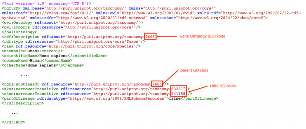
As an illustration, let’s look at how the taxonomy is represented in RDF. In the RDF listing, we see that taxonomy 9606 is defined as Homo Sapiens. Taxonomy 9606 is a subclass of taxonomy 9605, defined as Homininae. The subject is taxonomy 9606, the predicate is subclass and the object is taxonomy 9605. In addition, taxonomy 9606 has a narrower transitive relationship to taxonomy 63221, defined as Homo sapiens neanderthalensis, as well as taxonomy 741158, defined as Homo sapiens subsp. ‘Denisova’. Expressed in RDF terms, the subject is taxonomy 9606, the predicate is narrower transitive relationship and the objects are taxonomy 63221 and taxonomy 741158.
Example RDF file
Load the UniProt data
Instead of executing a large number of insert statements or other API calls, we use the Amazon Neptune Bulk Loader to load a subset of UniProt RDF files directly from the public S3 bucket.
Accessing the data
Before we can load data into the Neptune instance, we need an AWS Identity and Access Management (IAM) role that has access to the public bucket where the UniProt data resides. In addition, the Neptune loader requires a VPC endpoint for Amazon S3. For more information on bulk loading requirements, refer to the Neptune documentation on bulk loading. The IAM role and VPC endpoint have already been configured by our cloud formation template. We just need to define the role and endpoint settings.
Determine the files to load
The entire UniProt dataset is over 10 Terabytes uncompressed, and is growing rapidly. To save on time and cost, we only load the data that is relevant to our use case. Loading the complete UniProtKB will take around 74 hours, as the ingestion rate is around 6.6 GB per hour. The majority of loading cost is for the large DB writer instance. Using an r5.8xlarge, the cost is 6.46 USD per hour, so the cost of writing the entire UniProt dataset would be around 478 USD. For this example, we only load a single RDF file for Metazoa and the taxonomy and Gene Ontology files. This keeps our total loading time to under one hour, and the cost below 10 USD. These are the files to load: – taxonomy.rdf.gz – the taxonomy file – go.rdf.gz – the Gene Ontology file – uniprotkb_eukaryota_opisthokonta_metazoa_33208_0.rdf.gz – a single UniProtKB file for Metazoa
Execute the bulk load command
Now we have all the information needed to execute the bulk load command. In the following code, we define a function that: 1) Creates a json string of parameters required by the bulk loader command, 2) creates and sends an http request to the bulk loader endpoint, and 3) returns bulk load tracking IDs that will be used to track the loading process
We call this function for every file we wish to load. The entire loading process will take approximately 50 minutes. Times will vary depending on the region and the number and size of the datasets loaded.
Loading can also be accomplished with the %load command within the workbench. The load command works well for smaller files, but for loading large files, it makes it difficult to monitor the load process as it locks the entire notebook.
Monitor loading
Graph data comes in triples, which is the relationship between two nodes via an edge. Here are some metrics we captured during our previous load of the above files.
| File | File Size | Triples | Approximate Load Time in Seconds |
| taxonomy.rdf.gz | 50.5MB | 15950018 | 100 |
| go.rdf.gz | 3.3MB | 381392 | 10 |
| uniprotkb_eukaryota_opisthokonta_metazoa_33208_0.rdf | 3.45GB | 3.44E+08 | 1900 |
Here is an estimation for a full load of all supporting files and UniProtKB data:
| File Directory | Number of Files | Total File Size | Approximate Load Time |
| supporting/* | 16 | 8.2 GB | 1.25 hours |
| uniprot/* | 275 | 482 GB | 73 hours |
Loading can take some time, so it’s convenient to have a way to monitor the loading progress. The code below calls the Neptune endpoint with the load IDs we saved previously, and returns a status update on the bulk loading process for each file.
Downsize the Neptune instance
Once all the data is loaded, we no longer need a large writer instance, as we will mostly be reading from the database. It’s recommended that you resize the Neptune database to a smaller instance after you finish loading the files to save on running costs.
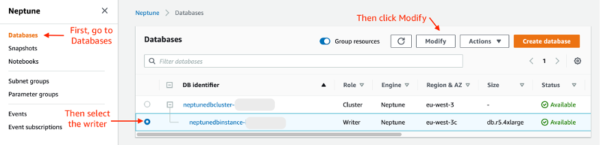
From the Neptune Console, go to Databases, choose the Neptune Writer, and click Modify.
Downsize Neptune step1
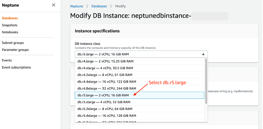
In the list of presented DB instance classes, select db.r5.large, the smallest instance available. Then click Continue.
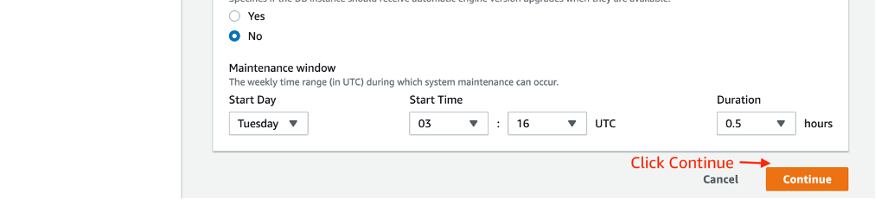
Downsize Neptune step 2
On the next page, choose Apply immediately, and click the Modify DB Instance button.
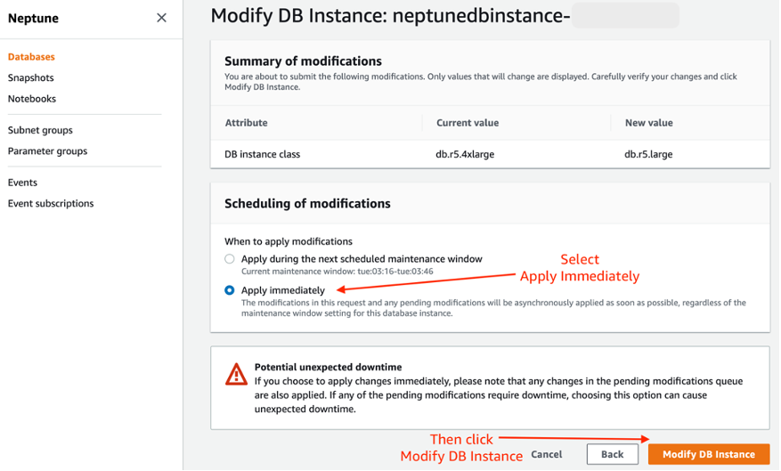
Downsize Neptune step 3
Your Neptune DB instance is now cost optimized for querying. For more information, refer to the steps in the Neptune Developer Guide.
Querying the UniProtKB
Now that we have the loaded the UniProt data, we can query it with SPARQL, a query language for graph data in RDF format. Amazon Neptune is compatible with SPARQL 1.1. If you are used to standard SQL queries, working with SPARQL should be familiar to you. A SPARQL query contains: Prefixes to abbreviate URIs; dataset declaration to specify the graphs being queried; SELECT clause that determines which attributes to return; WHERE clause that specifies matching criteria; and query modifiers for ordering results.
If you are unfamiliar with SPARQL queries, see Writing Simple Queries or the full guide in the SPARQL 1.1 Query Language documentation.
Next, we do some example queries to show how SPARQL works with UniProtKB.
Example 1: Simple Query
Let’s start with a simple query. In this query, we will look within the taxonomy tree, to see if there are any subclass records under Homo Sapiens. Homo Sapiens are coded with a taxonomy id of 9606. Query the web URI and scientific name of the subclass records.
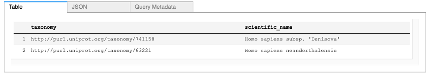
Example 1 results
The query returns two records, Homo Sapiens Neanderthalensis and Homo Sapiens Subsp. ‘Denisova’ , which are found under the taxonomy of Homo Sapiens. For taxonomy identifiers of other organisms, you may trace from the top node of cellular organisms.
Example 2: Query proteins and their related Gene Onotology (GO) code
Now, let’s find all the Homo Sapiens related proteins that have a Gene Ontology (GO) code. The Gene Ontology describes biological concepts with respect to molecular function, cellular components and biological processes. We will use the 9606 taxonomy code for “Homo Sapiens”. Instead of displaying the full IRI for each protein, use its mnemonic value. Since there are so many entries, we will also limit the query results to 10 rows.

Example 2 results
The query returns the proteins along with the respective GO IRI. Any proteins without a GO code will not be returned.
Example 3: Filter proteins by GO description
We can further filter the proteins by pattern matching its GO description. For this query, we will list all the Homo Sapiens proteins classified with “cholesterol biosynthetic process”. To do this, we add a filter condition containing a regular expression of the GO label. We will also parse the GO IRI so it is easier to read in the returned results.
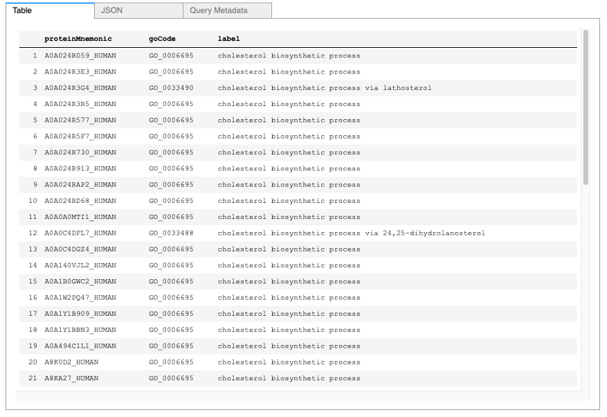
Example 3 results
We can also query the ancestor GO codes of proteins. Ancestor GO codes are represented by subclass relationships from a GO code to its ancestors. For example, GO code 0006695 is termed as the “cholesterol biosynthetic process” and has a subClassOf relation to the GO codes 0008203, termed the “cholesterol metabolic process”, and 1902653, termed the “secondary alcohol biosynthetic process”.
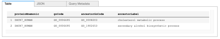
Example 4 results
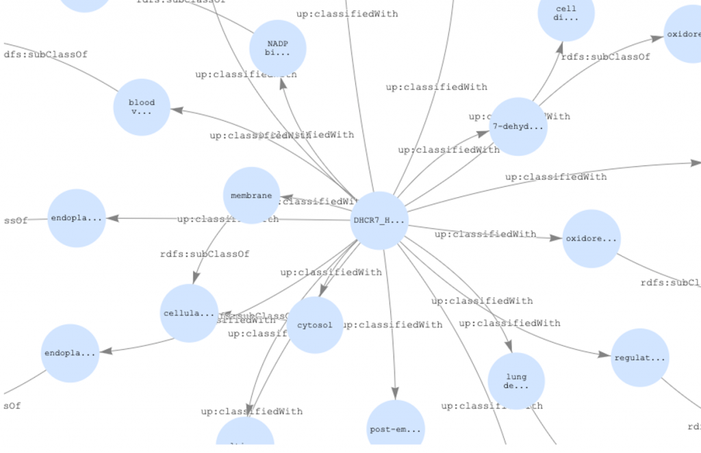
Example 5: Visualize a proteins Gene Ontology (GO)
To visualize the data for a protein in the “Graph” tab, we must construct a graph with the links between a protein and its GO codes and ancestor GO codes. We can create these relationships by using the CONSTRUCT operation which returns a graph with selected triples. For this example, we will only show 20 of the GO codes for the DHCR7 protein.

Example 5 results
Example 6: Adding data from Rhea to your Neptune Instance.
Rhea is an expert-curated knowledgebase of chemical and transport reactions of biological interest, and the standard for enzyme and transporter annotation in UniProtKB. In this example, use the public SPARQL endpoint of Rhea to enrich your Neptune instance with data from Rhea using the CONSTRUCT operation.
Starting with protein DHCR7_HUMAN, a reductase that catalyzes two reactions in the cholesterol biosynthetic pathway, we will demonstrate how to fetch the identifiers of all compounds that are metabolized by the enzyme (i.e. the chemical compounds of the enzyme-catalyzed reactions), and then create links between the protein in UniProtKB and the chemical compounds from Rhea.
The Rhea data is an external data store, so we use a federated query with the SERVICE keyword.

Example 6 results
Cleaning up
Be sure to delete you cloud formation template when you are finished and no longer need the Neptune DB to avoid incurring future costs.

Delete the CloudFormation template
Conclusion
In this example notebook, we have demonstrated some simple ways to create and use your own protein knowledgebase using the UniProt data available on AWS Open Registry of Data and Amazon Neptune. If you would like to explore further, try running this in your own account. Some other things to try would be joining to other graph databases using federated queries, querying features to train machine learning models, or inferring links with Neptune ML.
To learn more about Healthcare & Life Sciences on AWS, visit aws.amazon.com/health.