AWS Open Source Blog
Solving the Traveling Salesperson Problem with deep reinforcement learning on Amazon SageMaker
The Traveling Salesperson Problem (TSP) is one of the most popular NP-hard combinatorial problems in the theoretical computer science and operations research (OR) community. It asks the following question: “Given a list of cities and the distances between each pair of cities, what is the shortest possible route that visits each city exactly once and returns to the origin city?”
TSP has many important applications, such as in logistics, planning, and scheduling. The problem has been studied for decades, and many traditional optimization algorithms have been proposed to solve it, such as dynamic programming and branch-and-bound. Although these optimization algorithms are capable of solving TSP with dozens of nodes, it is usually intractable to use these algorithms to solve optimally above thousands of nodes on modern computers due to their exponential execution times.
In this article, we’ll show how to train, deploy, and make inferences using deep learning to solve the Traveling Salesperson Problem.
Overview
Recently, deep learning-based algorithms, such as graph neural networks (GNNs) along with reinforcement learning (RL), have been proposed to solve TSP. The advantages of the deep reinforcement learning algorithms are:
- Training a model from large synthetically (randomly) generated TSP instances.
- Generalization to new problems with different number of nodes.
- Quick inference time, relative to traditional optimization methods.
We are interested in applying open source TSP deep reinforcement learning algorithms in solving practical problems. In particular, we found the following capabilities important to successfully deploy RL-based solutions for supply chain operations:
- The ability to run model training distributed across multiple GPUs.
- The ability to host the model and provide routing in real time.
- The ability to interactively visualize the TSP solution to customers in order to receive feedback quickly.
Therefore, in this blog post, we will demonstrate:
- How to use Amazon SageMaker’s Distributed Data Parallel Library to train an open source deep learning-based TSP model across multiple GPUs.
- How to deploy the model to Amazon SageMaker inference endpoint. We also demonstrate how to perform batch inference.
- How to build a Streamlit interactive TSP demo using the SageMaker endpoint.
All the code can be found on GitHub.
Deep reinforcement learning TSP modeling
There are many options for designing the deep learning architecture for solving the Traveling Salesperson Problem. For this blog post, we will use a GNN to encode input nodes into dense feature vectors and use the Attention mechanism as a decoder to generate the ordered nodes in an autoregressive fashion.
- The idea behind a GNN is that stops included in the route can be thought of as nodes on a graph. The edge representation can be thought of as a measure of distance between the stops or whether stops exist within the predefined neighborhood region.
- The idea behind the Attention mechanism is to decode the routes in an autoregressive fashion by calculating the logit “attention” scores between nodes on the partial tour and the input nodes embedding.

Figure 1 shows the encoding and decoding processes based on Chaitanya Joshi’s repository. The dark gray rectangles during encoding represent various “fixed” embeddings projected from the original input—a set of nodes (Euclidean coordinates) and the nearest neighbor (NN) graph. The evolving state (the white box, bottom right), together with the fixed Node Embedding, is continuously projected onto the embedding known as Step Context (white rectangle) as the decoding process unfolds at a given step.
The State contains Node Embeddings of the first and last selected nodes in the partial tour. In this example, the first and fourth nodes’ Node Embeddings are included in the State. Fixed Context and Step Context are summed together to form the Query. Cross-product is performed between the Query and the Glimpse Key to form the Attention Score, which projects the Glimpse Values to the Logit Query.
Finally, another cross-product is performed between the Logit Key and the Logit Query to produce the final Logit Attention Score. This becomes the probability distribution from which the next unvisited node is drawn to join the partial tour.
The training approach utilizes the Reinforcement Learning Policy Gradient method called REINFORCE. The model training mechanics will look similar to the traditional Supervised Learning paradigm; however, there are a few key differences:
- Rather than calculating the loss in relationship to ground truth labels, the training tries to minimize the total tour length.
- Introducing a baseline learner to achieve faster convergence of the parameters during training. The baseline does not need to be created before training but can be incrementally updated during the training process itself.
- Rather than making “predictions” for each route, the model is actually creating a policy (that is, a sequence of consecutive decisions) that recommends which node to connect next given the partially formed tour and the set of unvisited nodes.
You can learn more about how REINFORCE algorithm works from the Policy Gradient REINFORCE Algorithm with Baseline tutorial or from Chapter 13 of Reinforcement Learning, Second Edition: An Introduction by Sutton and Barto.
Prepare scripts
Our model training code is modified from Chaitanya Joshi’s repository for the paper “Learning TSP Requires Rethinking Generalization.” The first step is to make the training distributed so that we can scale efficiently for training on large TSP datasets. The second step involves creating an endpoint that we can invoke to gain predictions in real time or in batch.
Training scripts
SageMaker’s Distributed Data Parallel Library extends SageMaker’s training capabilities on deep learning models with near-linear scaling efficiency, achieving fast time-to-train with minimal code changes. The library offers two options for distributed training: model parallel and data parallel. This guide focuses on how to train models using a data parallel strategy. We modify the script according to the example given in the SageMaker SDK documentation. First, we import the data parallel library:
Second, we wrap the model with the data distributed parallel object:
Third, we pin the GPUs to distinct processes:
Finally, we save the trained model only on the leader node. The leader node will have a synchronized model. This also avoids worker nodes overwriting the saved model and possibly corrupting the saved model.
The details of the training scripts can found on GitHub.
Inference scripts
For the Inference, we write a Python script that implements functions to load the model, preprocess input data, get predictions from the model, and process the output data in a model handler, according to the instructions from Adapting Your Own Inference Container—Amazon SageMaker.
The model_fn function is responsible for loading the model. It takes a model_dir argument that specifies where the model is stored as shown in the following example:
The input_fn function is responsible for deserializing the input data so that it can be passed to the model. It takes input data and content type as parameters and returns deserialized data as shown:
The predict_fn function is responsible for getting predictions from the model. It takes the model and the data returned from input_fn as parameters, and returns the prediction:
The output_fn function is responsible for serializing the data that the predict_fn function returns as a prediction to jsonline format:
The details of the inference scripts can be found on GitHub.
Distributed training of the ML model
After preparing the training and inference scripts, you can launch these scripts and get the TSP deep reinforcement learning model ready for use. Amazon SageMaker makes it possible to train deep learning models using deep learning frameworks, such as PyTorch, without the need to manage your own containers or training infrastructure. The SageMaker object used for running the training jobs is called an Estimator. Key arguments are included as follows:
instance_count: Increase this to train on multiple nodes (not merely multiple GPUs).distribution: This is what enables data distributed training.max_run:This specifies the max training time in seconds.
Using the following instance types in region US East 1, you can expect to pay approximately US$ 450, about 16 hours training. However, a pretrained model is included in the GitHub repository, if you do not want to reproduce model training yourself. Using this model, you can skip to the Inference section where you will deploy the model for inference.
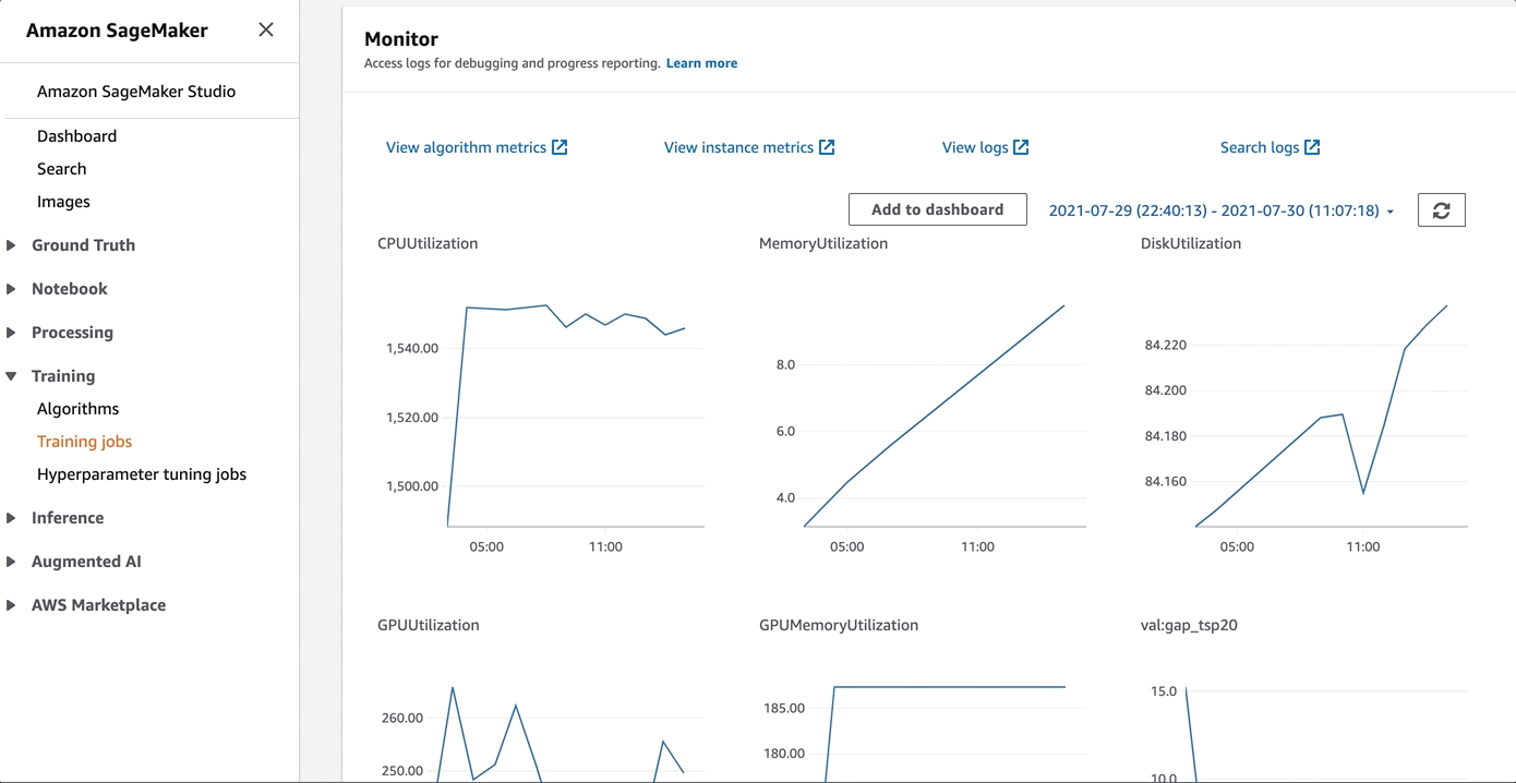
During the training, you can log on to the AWS Management Console to review a few training metrics as follows:
For details, refer to GitHub.
Inference
Test inference code locally
To test the inference code before deploying to the SageMaker endpoints, running the the code locally with some examples is worthwhile. First, we must load a pretrained model use the model_fn to see whether we can load the model properly:
Next we must use input_fn to see whether we can format the input to jsonlines:
Then we can call predict_fn to test that it is working fine:
Finally, we can use output_fn to see if it formats the output to jsonlines properly:
If you need to check whether it is working locally, you can further refactor the code to unit tests.
Deploy the inference code
After checking that the inference code is working properly, we can deploy the inference script and relevant source code to SageMaker endpoint, so the endpoint can provide real-time inference, as shown in the following example:
After the endpoint is deployed, you can call the endpoint to get the routing result:
Batch transform
Sometimes, you may need to route several TSP problems in a batch. You can use SageMaker Batch Transform to do this as shown:
For details, refer to GitHub.
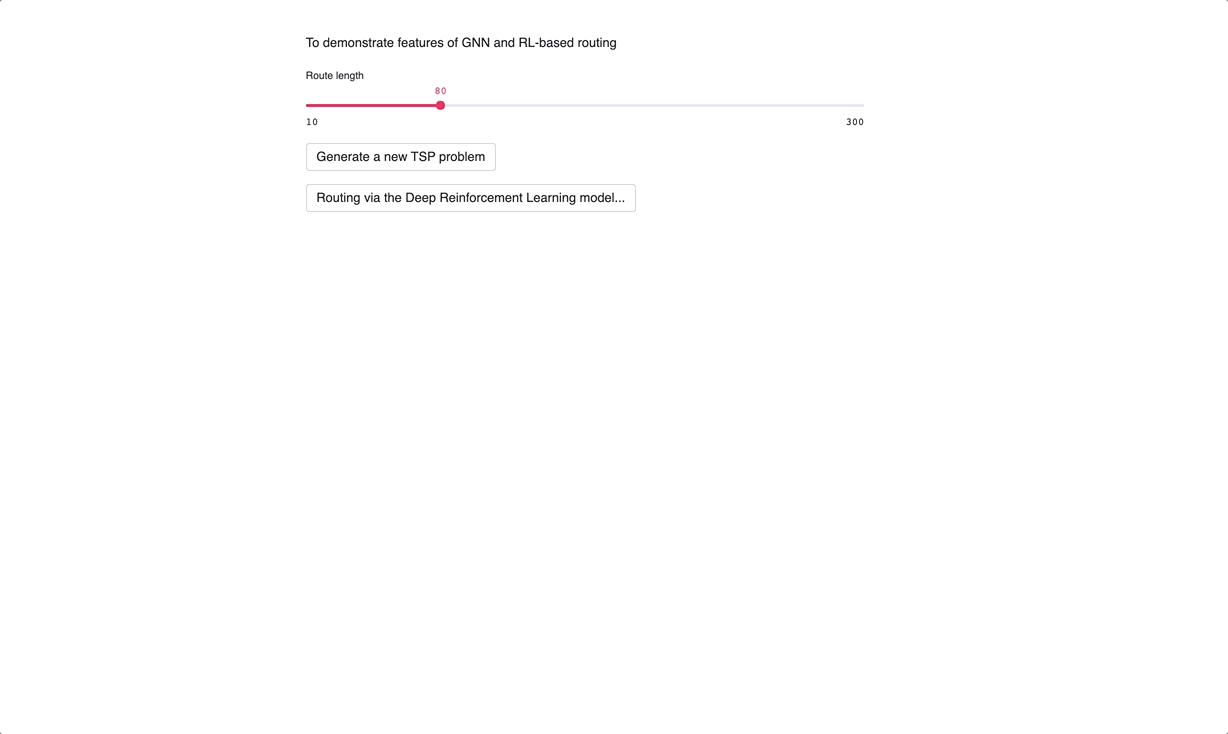
Demo and visualization
To better understand the model and for quick experimentation, we provide a simple Streamlit demo. To begin, you select a route length (that is, number of nodes). Then, you generate that number of nodes on a 2D plane. Finally, you pass the nodes to Amazon SageMaker to find the optimal route. This helps you to observe the performance of the routing algorithm at an intuitive level. A few things to look for:
- Nodes that are extremely close to each other should be visited in sequence.
- You don’t want to see a whole lot of “criss-crossing” on the graph. It should look like a single loop, not a spider web.
To run the demo, you can run the following steps on a SageMaker notebook instance.
Step 1: Update the Jupyter Notebook instance environment for hosting Streamlit.
This step configures and restarts the jupyter-server to host the streamlit application.
Step 2: Build the conda Python environment for the Streamlit app.
This step installs a conda environment specified in the environment.yaml file.
Step 3: Run the Streamlit app.
You should be able to view the app from:
Conclusion
Using deep learning and reinforcement learning to solve problems in optimization is still in its early days. However, remarkable progress has been made in a short period of time. In this blog post, we showed how to train, deploy, and make inferences using deep learning to solving the Traveling Salesperson Problem.